4. SciPy创建特殊矩阵
前边两章介绍的是如何创建matrix矩阵以及一些基本的操作运算函数,本章就一些特殊的矩阵以及特殊的方法继续介绍如何创建矩阵。
4.1 特殊的创建方法
在NumPy里、SciPy里有一些方法函数可以创建出比较特殊的矩阵。
4.1.1 mat和bmat函数
NumPy里可以通过mat、bmat等函数以数组作为形参来创建矩阵。
1). numpy.mat函数可将数组转为矩阵。
2). np.bmat函数可以矩阵为参数创建阵列的矩阵。
import numpy as np
a = np.mat(np.ones([3, 3]))
b = np.mat(np.zeros([3,3]))
print a,"#a"
print b,"#b"
c = np.bmat("a,b;b,a")
print c,"#c"
程序执行结果:
[[ 1.  1.  1.]
 [ 1.  1.  1.]
 [ 1.  1.  1.]] #a
[[ 0.  0.  0.]
 [ 0.  0.  0.]
 [ 0.  0.  0.]] #b
[[ 1.  1.  1.  0.  0.  0.]
 [ 1.  1.  1.  0.  0.  0.]
 [ 1.  1.  1.  0.  0.  0.]
 [ 0.  0.  0.  1.  1.  1.]
 [ 0.  0.  0.  1.  1.  1.]
 [ 0.  0.  0.  1.  1.  1.]] #c
4.1.2 tile函数
tile函数的功能有点像楼宇建设里的铺地面转的工作,将tile的第一参数(瓷砖)铺第二个参数指定的行和列m x n那么大一块。
import numpy as np
t = np.arange(9).reshape([3, 3])
tm = np.tile(t, [3,2])
print tm
程序执行结果
[[0 1 2]
 [3 4 5]
 [6 7 8]] #t
[[0 1 2 0 1 2]
 [3 4 5 3 4 5]
 [6 7 8 6 7 8]
 [0 1 2 0 1 2]
 [3 4 5 3 4 5]
 [6 7 8 6 7 8]
 [0 1 2 0 1 2]
 [3 4 5 3 4 5]
 [6 7 8 6 7 8]] #tm
4.1.3 block_diag函数
scipy.linalg.block_diag函数可以创建一个广义“主对角线”非0的大矩阵,其参数是矩阵,用矩阵作为主对角线性的值,所以矩阵会比较的大。
import numpy as np
import scipy.linalg as sl
a = np.mat(np.ones([3, 3]))
b = np.mat(np.ones([4,3]))
c = np.mat(np.ones([3,4]))
print a,"#a"
print b,"#b"
print c,"#c"
d = sl.block_diag(a,b,c)
print d,"#d"
程序执行结果:
[[ 1.  1.  1.]
 [ 1.  1.  1.]
 [ 1.  1.  1.]] #a
[[ 1.  1.  1.]
 [ 1.  1.  1.]
 [ 1.  1.  1.]
 [ 1.  1.  1.]] #b
[[ 1.  1.  1.  1.]
 [ 1.  1.  1.  1.]
 [ 1.  1.  1.  1.]] #c
[[ 1.  1.  1.  0.  0.  0.  0.  0.  0.  0.]
 [ 1.  1.  1.  0.  0.  0.  0.  0.  0.  0.]
 [ 1.  1.  1.  0.  0.  0.  0.  0.  0.  0.]
 [ 0.  0.  0.  1.  1.  1.  0.  0.  0.  0.]
 [ 0.  0.  0.  1.  1.  1.  0.  0.  0.  0.]
 [ 0.  0.  0.  1.  1.  1.  0.  0.  0.  0.]
 [ 0.  0.  0.  1.  1.  1.  0.  0.  0.  0.]
 [ 0.  0.  0.  0.  0.  0.  1.  1.  1.  1.]
 [ 0.  0.  0.  0.  0.  0.  1.  1.  1.  1.]
 [ 0.  0.  0.  0.  0.  0.  1.  1.  1.  1.]] #d
4.2 特殊矩阵
以scipy.linalg提供的一些特殊矩阵创建函数为例。
1).scipy.linalg.pascal创建杨辉三角矩阵。
import scipy.linalg
x = scipy.linalg.pascal(7)
print x
执行结果
[[  1   1   1   1   1   1   1]
 [  1   2   3   4   5   6   7]
 [  1   3   6  10  15  21  28]
 [  1   4  10  20  35  56  84]
 [  1   5  15  35  70 126 210]
 [  1   6  21  56 126 252 462]
 [  1   7  28  84 210 462 924]]
看主对角线两侧就是杨辉三角的数据。
2). scipy.linalg.leslie创建莱斯利矩阵。
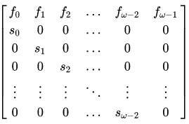
w维向量$f_w= (f_0,f_1,\dots,f_{w-1})$作为第一个参数而w-1维向量$s_{w-1} = (s_0,s_1,\dots,s_{w-2})$作为第二个参数,结果是$w \times w$维的矩阵。
import scipy.linalg
import numpy
f = numpy.array([0.3, 0.1, 0.4, 0.2])
s = numpy.array([0.2, 0.8, 0.7])
l = scipy.linalg.leslie(f, s)
print l
程序执行结果:
[[ 0.3  0.1  0.4  0.2]
 [ 0.2  0.   0.   0. ]
 [ 0.   0.8  0.   0. ]
 [ 0.   0.   0.7  0. ]]
3). scipy.linalg.hilbert希尔伯特矩阵,特点是某位置上的数值是该位置的行坐标加列坐标加一的倒数。
import scipy.linalg
h = scipy.linalg.hilbert(4)
print h
程序执行结果:
[[ 1.          0.5         0.33333333  0.25      ]
 [ 0.5         0.33333333  0.25        0.2       ]
 [ 0.33333333  0.25        0.2         0.16666667]
 [ 0.25        0.2         0.16666667  0.14285714]]
4). scipy.linalg.hankel汉克尔矩阵每条副对角线上的值相同,与常对角矩阵Toeplitz矩阵类似,将汉克尔矩阵上下颠倒即可得到每一条主对角线的元素都相等的Toeplitz矩阵。
import scipy.linalg
h1 = scipy.linalg.hankel([1, 17, 99])
print h1, "#h1"
h2 = scipy.linalg.hankel([1, 2, 3], [4, 5])
print h2, "#h2"
h3 = scipy.linalg.hankel([1, 2, 3], [3, 4, 5])
print h3, "#h3"
h4 = scipy.linalg.hankel([1, 2, 3], [2, 3, 4, 5])
print h4, "#h4"
h = scipy.linalg.hankel([1, 2, 3], [1, 2, 3, 4, 5])
print h
h5 = scipy.linalg.hankel([1, 2, 3], [1, 2, 3, 4, 5, 6])
print h5, "#h5"
h6 = scipy.linalg.hankel([1, 2, 3, 4], [1, 2, 3, 4, 5])
print h6, "#h6"
程序执行结果:
[[ 1 17 99]
 [17 99  0]
 [99  0  0]] #h1
[[1 2]
 [2 3]
 [3 5]] #h2
[[1 2 3]
 [2 3 4]
 [3 4 5]] #h3
[[1 2 3 3]
 [2 3 3 4]
 [3 3 4 5]] #h4
[[1 2 3 2 3]
 [2 3 2 3 4]
 [3 2 3 4 5]]
[[1 2 3 2 3 4]
 [2 3 2 3 4 5]
 [3 2 3 4 5 6]] #h5
[[1 2 3 4 2]
 [2 3 4 2 3]
 [3 4 2 3 4]
 [4 2 3 4 5]] #h6
5).scipy.linalg.toeplitz每条主对角线上的值均相等。
from scipy.linalg import toeplitz
print toeplitz([1,2,3], [1,4,5,6])
程序执行结果:
[[1 4 5 6]
 [2 1 4 5]
 [3 2 1 4]]